You are here
The use of modelling tools to assess local scale inundation and erosion risk
This web content was produced by Jeff Hansen, School of Earth and Environment, University of Western Australia.
Please cite as:
Hansen, J.E., 2016: The use of modelling tools to assess local scale inundation and erosion risk. CoastAdapt, National Climate Change Adaptation Research Facility, Gold Coast.
At a glance
- Models can provide a detailed view of coastal inundation and erosion risk across a range of spatial scales and under a range of climate and storm scenarios. The complexity of most models, as well as the input data required, limits their use to specific areas.
- Local scale modelling should only be conducted following a preliminary risk assessment that specifically identifies local areas that are vulnerable due to geomorphology (e.g. low lying) or include high value infrastructure.
- We describe two types of models: empirical and process-based numerical models. Each type of model has distinct advantages and disadvantages. Which should be applied will depend on the location, available resources, and the time horizon being considered.
Main text
Why use models?
Historically, a simple bathtub or bucket-fill approach has been used to assess coastal inundation and associated erosion risk from rising sea levels. This approach has assumed that a (for example) 1 m rise in sea level will inundate all locations at or below an elevation of 1 m plus the highest astronomical tide. This approach is a relatively simple and efficient means of identifying areas likely to be at risk and has recently been completed for much of Australia’s populated coastal areas (see http://coastalrisk.com.au/).
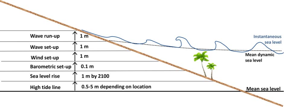
However, the bathtub approach neglects the dynamic components of sea level that can further increase sea levels. It provides no information on the amount of shoreline erosion other than the shoreline recession due to the increase sea level alone. Sea levels fluctuate on a number of time scales, from seconds to weeks associated with a range of processes in the ocean. In addition to tides, sea levels vary due to waves (set-up and run-up), storm surge (wind driven and barometric set-up) and changes in ocean circulation. Each of these processes can increase sea level by tens of centimetres to more than a metre (Figure 1). Thus, while adequate in some areas, the bathtub approach may understate the risk of coastal inundation in other areas.
T3W1_Figure-1.jpg
The physical processes that result in these dynamic sea level variations are generally well understood and included in a range of models. As a result, models can provide a detailed local scale assessment of inundation risk. Similarly, a range of models can be used to understand erosion risk as a result of climate change. In many numerical models erosion (and accretion) can be modelled simultaneously with inundation, or erosion can be modelled independently using empirical relationships between numerically modelled or statistically derived physical forcing (e.g. waves and winds) and erosion. Predictions of erosion risk will generally be less accurate than inundation predictions due to the inherent complexity of sediment transport, but a range of models can still provide detailed and useful information on areas that are likely to erode in response to climate change.
Overview of models
There are two primary classes of models for predicting coastal inundation and erosion; these are empirical, or data driven, and process-based numerical models.
Empirical models are created by developing a mathematical model that best reproduces a set of observations; the model can then be used predictively. For example, empirical models have been created to predict wave run-up from offshore wave height and beach slope. A key feature of most empirical models is they do not account for the relevant physical processes directly; rather the relevant processes are implicitly included in the derived empirical relationship. An advantage of empirical models is they are relatively simple and easy to apply. The main disadvantage is developing them requires extensive observations which also means they are specific to the sites at which they were developed or to sites with similar morphology.
Process-based numerical models consider the relevant physical processes and the resulting inundation and erosion. (A good overview of numerical models is provided here: http://www.coastalwiki.org/wiki/Process-based_modelling). For the coast, these processes include wave propagation, growth due to wind, wave breaking, as well as the currents and sea level variations (see Figure 1). Process-based numerical models can also be applied to estuary environments in which rising sea levels may alter estuary area, tidal circulation and dynamics, salinity, and fresh water inputs, making areas more or less likely to experience inundation and erosion.
Process-based models, while not perfect, provide a range of advantages, particularly that the results are directly related to the site being modelled. These models can range in complexity, from predicting wave height and set-up across a simple cross-shore transect, to predicting inundation within an estuary using a three-dimensional coastal model that includes wind, waves, salinity, and atmospheric pressure. However the complexity of these models is also their main disadvantage; generally the modelling and analysis will require personnel with specific training and experience.
Another disadvantage is their need for detailed input conditions. For example, without reasonably detailed bathymetry, numerical predictions of inundation and erosion are unlikely to be accurate enough to warrant the cost and effort required. Most modern coastal and estuarine numerical models also include sediment transport modules that can estimate erosion and accretion over a range of spatial and temporal scales. However, the sediment transport formulations can be prone to error (see Amoudry and Souza 2011 for a review).
Often, empirical and process-based models are combined to take advantage of their respective strengths. For example, the output of a number of process-based numerical simulations can be used as the basis of an empirical probabilistic model of inundation and erosion; or an empirical statistical model can be used to generate the input conditions for a process-based numerical model (e.g. Callaghan et al. 2008).
When to use models
Given their complexity and input requirements, it is often impractical to use detailed models across large spatial scales. Instead, it is more practical to do a first-pass assessment using existing bathtub inundation predictions under different sea-level rise scenarios to identify areas where a numerical model can provide additional information on inundation and erosion risk. For example, for a high relief coastline fronted by stable sea cliffs, the bathtub approach may be sufficient with little gained from modelling.
There are a number of data sources available in Australia to support a first pass assessment:
- CoastAdapt has inundation mapping for each coastal local council in Australia, for 2050 and 2100, and two scenarios of greenhouse gas concentrations, see CoastAdapt datasets 2: future sea-level rise and its effect on coastal inundation;
- For a wider range of sea-level rise scenarios, inundation modelling results are available from the Coastal Risk Australia website http://coastalrisk.com.au.
In both datasets, inundation mapping is only available where LiDAR surveys have been carried out.
A more detailed model can be used in low-lying coastal and estuarine areas where detailed information will help assess communities or structures at risk, locations where additional inundation may alter the mitigation strategy, or locations identified to be at risk by regional scale modelling.
Any local scale erosion modelling will also need to consider regional sediment transport patterns and sediment availability, and these will change as a result of climate change. For example, a decrease in rainfall may result in a decrease in sediment delivered to estuaries and the coast from catchments, resulting in erosion irrespective of sea level changes. The likely impacts of climate change on Australia’s coastline are described in Sediment compartments for coastal management and Guidelines on using Expert knowledge on coastal compartments. This information can be used in concert with any local scale modelling.
What data are needed to run models and what is available?
For areas or locations where modelling will provide additional detail, there needs to be sufficient data available to initialise the models. Numerical models, in particular, rely on bathymetry/topography at a high enough spatial resolution to resolve features that will impact the waves, currents, tides and ultimately the inundation and erosion. Generally this will be gridded elevation data with a resolution of ~5-25 m. A LiDAR based 5 m digital elevation model of topography is available from Geoscience Australia for many areas (available here: http://www.ga.gov.au/elvis/). Bathymetry is generally harder to obtain, but information from aerial (LiDAR), multi beam or single beam surveys are held by State and the Commonwealth (Geoscience Australia) for some areas. For example, the Western Australia state government has collected aerial LiDAR bathymetry available at 5 m resolution for much of the Perth metro and surrounding area.
Accurate bathymetry in shallow water is critical for realistic predictions of inundation and erosion using both empirical and process-based models. Therefore collecting these data in areas deemed to be high-risk by the first-pass analysis may be required. This is particularly true in estuaries where increasing sea levels will alter the estuary area, geometry and corresponding tidal dynamics, which will subsequently impact areas subject to inundation and erosion. For deeper waters (>50 m) a ~250 m grid is available from Geoscience Australia (http://www.ga.gov.au/metadata-gateway/metadata/record/gcat_67703).
Environment conditions are required to drive both empirical and process-based models. It is impractical to run any type of model over long periods of time to understand coastal inundation and erosion, therefore methodologies have been developed to statistically synthesize a vast array of variables (i.e. combinations of wave height, rainfall, wind speed, storm sequences etc.) into a subset of conditions likely to cause the most inundation and erosion. This often involves developing synthetic conditions using statistical models based on time series of observed or predicted conditions (e.g. Callaghan et al. 2008; Ranasinghe et al. 2012). The advantage of synthetic conditions is that they can be based on historic extreme events or on expected average return interval (ARI) events under a range of climate scenarios.
Available models and limitations
A vast array of empirical models exists with most developed and tailored to produce a specific output (e.g. shoreline erosion). Two examples of relevant empirical models include those by:
- Stockdon et al. (2006), which predicts wave set-up and run-up using offshore wave height, wave period and beach slope; and
- Hapke and Plant (2010) that probabilistically predicts coastal cliff erosion.
However, as empirical models do not explicitly model physical processes they are only relevant at the sites they were developed, or at those with very similar morphology. For example, a commonly used empirical model for coastal recession due to rising sea levels is the Bruun rule (Bruun 1962), which essentially predicts that the coastal profile will maintain a constant shape and will just migrate landward to accommodate rising sea level. However, the Bruun rule assumes an entirely sandy coast backed by dunes and thus would be completely inappropriate to apply along rocky or reef coasts. See also Rules of thumb.
The performance of process-based numerical models at predicting inundation and erosion has improved in recent decades. Examples of commonly used process-based numerical models include:
- Delft3D (https://www.deltares.nl/en/software/delft3d-4-suite/) coupled with the wave model SWAN (http://www.swan.tudelft.nl/),
- XBeach (http://oss.deltares.nl/web/xbeach/) and
- Mike21 (https://www.mikepoweredbydhi.com/products/mike-21), (all sites accessed 6 June 2016).
Each of these models operates differently but all are capable of predicting inundation and erosion. As process-based numerical models explicitly account for a range of processes, they can be applied in a wider range of environments (e.g. rocky and sandy coasts). Similar to empirical models however, it is important to select a numerical model that considers processes that are likely to be important. For example, XBeach does not account for salinity variations and so it would be an inappropriate model to use in an estuarine environment.
Once a model is selected and set up it will need to be calibrated and validated using observations to ensure realistic predictions are being made. This may include comparing predicted waves, currents, and shoreline erosion with conditions observed during a large storm. The complexity and computational infrastructure required to run numerical models and interpret their results will generally require contracting consulting companies or universities with expertise in modelling.
Examples of using modelling to assess inundation and erosion risk
An example of the use of models to assess coastal inundation and erosion risk is that of the Coastal Storm Modelling System (CoSMoS, see http://walrus.wr.usgs.gov/coastal_processes/cosmos/index.html and Barnard et al. 2014) established along portions of the California (USA) coastline by the US Geological Survey. The CoSMoS example outlines a comprehensive approach to estimate coastal inundation and erosion risk. CoSMoS uses a nested modelling system whereby different process-based numerical models are run sequentially with each providing the boundary conditions to subsequent models. Although complex, this approach captures the physical links between the larger scale processes (e.g., in Australia, an East Coast Low in the Tasman Sea) and local-scale inundation and erosion, and therefore will give the most realistic assessment of inundation and erosion risk.
The nested approach begins by creating regional (~100 km scale) wind and wave boundary conditions for historic and projected conditions. Historical conditions are derived from direct observations (e.g. wave buoys and weather stations) as well as global coupled ocean-atmosphere numerical simulations available for previous decades (reanalysis products, see http://www.ecmwf.int/en/research/climate-reanalysis). Historical conditions are useful for model calibration/validation as well as for evaluating model performance from past events that led to coastal inundation and erosion. Predictions of future wind, atmospheric pressure and waves are available from global ocean-atmosphere models based on a range of the Intergovernmental Panel on Climate Change (IPCC) CO2 emissions and concentration scenarios (see https://researchdata.ands.org.au/cawcr-global-wind-climate-projections/625616). These are used to develop projected annual, 20 and 100 year ARI events. As climate change is expected to alter storm tracks and characteristics, in many locations it is expected that the historical ARI events are likely to differ from the projected events.
The regional wave, water level, wind and atmospheric pressure conditions produced from the global models are then used as boundary conditions for a higher resolution coupled circulation-wave model (e.g. Delft3D coupled with SWAN) that extends to offshore of the continental shelf break (~100 m depth) and has an intermediate resolution (~25-250 m). The coupled wave-flow model propagates waves onshore while also including wind growth of waves, currents and atmospheric set up.
The regional model then provides the boundary conditions for local-scale models that cover the area(s) identified to be at most risk in the first-pass assessment. These local models will have a higher resolution (~5-15 m), needed to adequately resolve the wave and wind setup at the shoreline, and thus provide better predictions of inundation.
CoSMoS uses Delft3D and SWAN for the regional models and XBeach for the local models. XBeach has the advantage that it includes wave run-up from infragravity waves (waves with periods of 30-300 seconds that account for the largest amount of run-up at the shoreline). An advantage of the nested approach is that once the modelling system has been set up, it is relatively easy to add additional local area models.
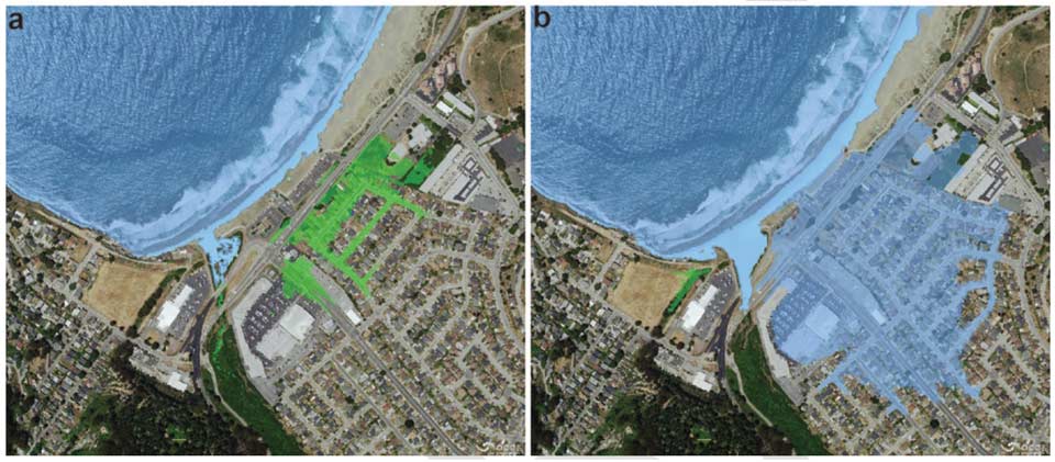
Using the nested approach, CoSMoS has produced inundation and erosion maps for portions of the California coast and compiled the output into a publically available web tool (http://data.prbo.org/apps/ocof/, Ballard et al. 2014). This allows inundation, wave heights, currents and duration to be examined under a range of different sea-level rise scenarios coupled with projected ARI storm events. Example output from CoSMoS from Pacifica, California, is shown in Figure 2 considering a 1.25 m static rise in sea level (Figure 2a) as well as with a 1.25 m rise in sea level plus the projected 20 year ARI storm (Figure 2b). In this example including the wave and atmospheric effects results in considerably more inundation than the bathtub approach.
T3W1_Figure-2.jpg
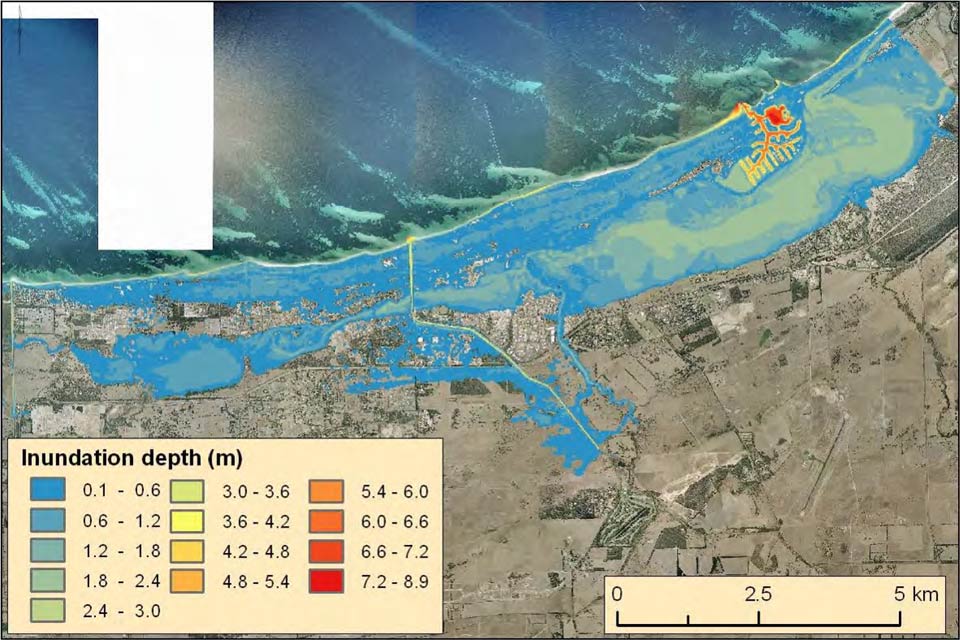
A similar approach was undertaken by Martin et al. (2014) to investigate projected inundation and erosion for Busselton, Western Australia, under a range of climate scenarios. In this case the inundation was predicted using process-based numerical models (GCOM2D and ANUGA) with numerous combinations of sea-level rise, riverine flooding, and increased tidal water levels due to a cyclone modelled after Tropical Cyclone Alby, which hit the area in 1978. In this example, shoreline erosion was modelled over a range of time horizons (out to 2300) empirically considering rising sea levels, sediment supplies, and substrate. Unlike the CoSMoS example, erosion was modelled independently of inundation in order to incorporate regional scale variability in sediment supply and substrate, which may dominate shoreline erosion patterns farther in the future (>2100). Similar to the CoSMoS example, the inclusion of storm conditions results in considerably more inundation than that from sea-level rise alone (Figure 3).
T3W1_Figure-3.jpg
Further information
Barnard, P.L., and Coauthors, 2009: The framework of a coastal hazards model; a tool for predicting the impact of severe storms, U.S. Geological Survey Open-File Report 2009-1073. Accessed 28 May 2016. [Available online at http://pubs.usgs.gov/of/2009/1073/].
Bowen, A.J., D.L. Inman, and V.P. Simmons, 1968: Wave 'set-down' and set-up. Journal of Geophysical Research, 73(8), 2569-2577.
Dee, D.P., and Coauthors, 2011: The ERA-Interim reanalysis: configuration and performance of the data assimilation system. Quarterly Journal of the Royal Meteorological Society, 137(656), 553-597.
Feng, M., M.J. McPhaden, S.-P. Xie, and J. Hafner, 2013: La Niña forces unprecedented Leeuwin Current warming in 2011. Scientific Reports, 3, 1277.
Hemer, M.A., J. Katzfey, and C.E. Trenham, 2013: Global dynamical projections of surface ocean wave climate for a future high greenhouse gas emission scenario. Ocean Modelling, 70, 221-245.
Woodroffe, C.D., and Coauthors, 2012: Approaches to risk assessment on Australian coasts: A model framework for assessing risk and adaptation to climate change on Australian coasts. National Climate Change Adaptation Research Facility, Gold Coast, 205 pp. Accessed 28 May 2016. [Available online at https://www.nccarf.edu.au/publications/approaches-risk-assessment-australian-coasts].
Source material
Amoudry, L.O. and Souza, A.J., 2011. Deterministic coastal morphological and sediment transport modeling: a review and discussion. Reviews of Geophysics, 49(2): RG2002.
Ballard, G., P.L. Barnard, L. Erikson, M. Fitzgibbon, K. Higgason, M. Psaros, S. Veloz, and J. Wood, 2014: Our Coast Our Future (OCOF). Petaluma, California. Accessed 28 May 2016. [Available online at www.pointblue.org/ocof].
Barnard, P.L., M. Ormondt, L.H. Erikson, J. Eshleman, C. Hapke, P. Ruggiero, P.N. Adams, and A.C. Foxgrover, 2014: Development of the Coastal Storm Modeling System (CoSMoS) for predicting the impact of storms on high-energy, active-margin coasts. Natural Hazards, 74(2), 1095-1125.
Bruun, P., 1962: Sea-level rise as a cause of shore erosion. Journal of the Waterways and Harbors division, 88(1), 117-132.
Callaghan, D.P., P. Nielsen, A. Short, and R. Ranasinghe, 2008: Statistical simulation of wave climate and extreme beach erosion. Coastal Engineering, 55(5), 375-390.
Hapke, C., and N. Plant, 2010: Predicting coastal cliff erosion using a Bayesian probabilistic model. Marine Geology, 278(1–4), 140-149.
Martin, S., D. Moore, and M. Hazelwood, 2014: Coastal inundation modelling for Busselton, Western Australia, under current and future climate. Record 2014/03. Geoscience Australia: Canberra. Accessed 28 May 2016. [Available online at http://dx.doi.org/10.11636/Record.2014.003].
Ranasinghe, R., D. Callaghan, and M.J.F. Stive, 2012: Estimating coastal recession due to sea level rise: beyond the Bruun rule. Climatic Change, 110(3-4), 561-574.
Stockdon, H.F., R.A. Holman, P.A. Howd, and J.A.H. Sallenger, 2006. Empirical parameterization of setup, swash, and runup. Coastal Engineering, 53(7), 573-588.